User Guide
Installation
pyquafu requires python>=3.8. And it’s suggested to activate an
individual virtual environment for it, see for axample
quafu-tutorial-venv.
For the latest stable version, run the following codes in the command line/terminal:
pip install pyquafu
Set up your Quafu account
If you haven’t have an account, you may register on the
Quafu website at first. Then you will
find your apitoken <your API token> on the Dashboard page,
which is required when you send tasks to ScQ-chips.
By executing the following codes your token will be saved to your local device.
from quafu import User
user = User("<your API token>")
user.save_apitoken()
Once you’ve done this, you may look over the available ScQ-chips in the experimental backends.
available_backends = user.get_available_backends()
system_name      qubits  status
ScQ-P10          10      Offline
ScQ-P18          18      None Status
Baiwang          136     Online
ScQ-P102         102     Offline
ScQ-P10C         10      Maintenance
Miaofeng         108     Online
Dongling         106     Online
Haituo           105     Online
Baihua           118     Online
Yunmeng          156     Online
Xiang            35      Offline
Note: The next time you visit pyquafu, you don’t have to save the
token again. Yet a quafu token is not permanently validating, from time
to time you may click ``refresh`` to get a new one on
Quafu webpage .
Build your first quantum circuit
Let’s start by initializing a circuit with 5 qubits,
import numpy as np
from quafu import QuantumCircuit

qc = QuantumCircuit(5)
Apply Gates
PyQuafu supports ‘qc.name(args)’ style to apply gates and also
other instructions.
qc.x(0)
qc.x(1)
qc.cnot(2, 1)
qc.ry(1, np.pi/2)
qc.rx(2, np.pi)
qc.rz(3, 0.1)
qc.cz(2, 3)
<quafu.circuits.quantum_circuit.QuantumCircuit at 0x1ffda5f5ad0>
Alternatively, you may manually instantiate a gate and add it to the circuit.
# equivalent to qc.x(0)
from quafu.elements.element_gates import *
gate = XGate(pos=0)
qc.add_gate(gate)
# you may also use the left shift operator
# qc << XGate(pos=0)
This is actually what .name(args) functions do. You would find
the second style convenient when build a new circuit from existing one.
For quantum gates Quafu supports, please check the API reference for Quantum Circuit
or use python-buitin dir() method.
print(dir(qc))
['__class__', '__delattr__', '__dict__', '__dir__', '__doc__', '__eq__', '__format__', '__ge__', '__getattribute__', '__getstate__', '__gt__', '__hash__', '__init__', '__init_subclass__', '__le__', '__lt__', '__module__', '__ne__', '__new__', '__reduce__', '__reduce_ex__', '__repr__', '__setattr__', '__sizeof__', '__str__', '__subclasshook__', '__weakref__', '_used_qubits', 'add_gate', 'add_pulse', 'barrier', 'circuit', 'cnot', 'cp', 'cs', 'ct', 'cx', 'cy', 'cz', 'delay', 'draw_circuit', 'fredkin', 'from_openqasm', 'gates', 'h', 'id', 'iswap', 'layered_circuit', 'mcx', 'mcy', 'mcz', 'measure', 'measures', 'num', 'openqasm', 'p', 'plot_circuit', 'rx', 'rxx', 'ry', 'ryy', 'rz', 'rzz', 's', 'sdg', 'sw', 'swap', 'sx', 'sxdg', 'sy', 'sydg', 't', 'tdg', 'to_openqasm', 'toffoli', 'unitary', 'used_qubits', 'w', 'x', 'xy', 'y', 'z']
Measure
Add measurement information including qubits measured (measures) and
the classical bits keeping the measured results (cbits). If there is
no measurement information provided, all qubits are measured by default.
measures = [0, 1, 2, 3, 4]
cbits = [0, 1, 2, 4, 3]
qc.measure(measures,  cbits=cbits)
qc.measures
{0: 0, 1: 1, 2: 2, 3: 4, 4: 3}
Visualize
From version=0.3.2, PyQuafu provides two similiar ways to
visualize quantum circuits. You can draw the circuit using the
draw_circuit method and use width parameter to adjust the length of the circuit.
qc.draw_circuit(width=4)
q[0]  ------X--------X-------------------- M->c[0]

q[1]  ------X--------+----RY(1.571)------- M->c[1]
                     |
q[2]  ---------------*----RX(3.142)----*-- M->c[2]
                                       |
q[3]  --RZ(0.100)----------------------Z-- M->c[4]

q[4]  ------------------------------------ M->c[3]
Alternatively, you may create a figure by
qc.plot_circuit(title='A Quantum Circuit')
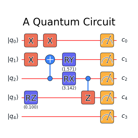
The latter visualization uses matplotlib as the backend and you may
save the figure as any format that matplotlib supports.
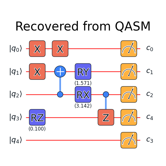
OPENQASM Support
pyquafu is backward compatible with quantum gates in
OPENQASM2.0. You can store your
quantum circuit as openqasm string, and also initialize your quantum
circuit with openqasm text.
qasm = qc.to_openqasm()
print(qasm)
OPENQASM 2.0;
include "qelib1.inc";
qreg q[5];
creg meas[5];
x q[0];
x q[1];
cx q[2],q[1];
ry(1.5707963267948966) q[1];
rx(3.141592653589793) q[2];
rz(0.1) q[3];
cz q[2],q[3];
x q[0];
measure q[0] -> meas[0];
measure q[1] -> meas[1];
measure q[2] -> meas[2];
measure q[3] -> meas[4];
measure q[4] -> meas[3];
del qc
qc = QuantumCircuit(5)
qc.from_openqasm(qasm)
qc.plot_circuit('Recovered from QASM')
Parameter
Execution and Simulation
Now you are ready to submit the circuit to the experimental backend. First, initialize a Task object
from quafu import Task
task = Task()
You can configure your task properties using the
config method. Here we
choose the backend (backend) as ScQ-P18, the single shots number
(shots) as 2000 and compile the circuit on the backend
(compile).
task.config(backend="ScQ-P18", shots=2000, compile=True)
If you set the compile parameter to False, make sure that you
know the topology of the backend well and submit a valid circuit.
Send the quantum circuit to the backend and wait for the results.
Note that, by default the wait option is set to be False, which
means that you need use the retrieve method to fetch results when task is done.
res = task.send(qc)
# After task is done, you could fetch results as below
res = task.retrieve(<your-task-id>)
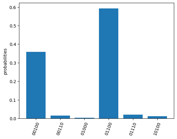
You can use the returned results to check the count and probability of each measured bit string. The output bits are arranged in big-endian convention by default, see also the next sectioin.
print(res.counts) #counts
print(res.probabilities) #probabilities
res.plot_probabilities()
OrderedDict([('00100', 717), ('00110', 31), ('01000', 6), ('01100', 1185), ('01110', 39), ('10100', 22)])
{'00100': 0.3585, '00110': 0.0155, '01000': 0.003, '01100': 0.5925, '01110': 0.0195, '10100': 0.011}
png
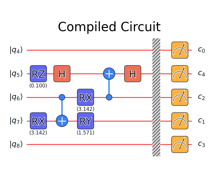
The returned results contain also the compiled circuit, from which you may find optimization was made.
res.transpiled_circuit.plot_circuit("Compiled Circuit")
If you want to check the correctness of the executed results. Quafu provide simple circuit similator
from quafu import simulate
simu_res = simulate(qc)
simu_res.plot_probabilities()
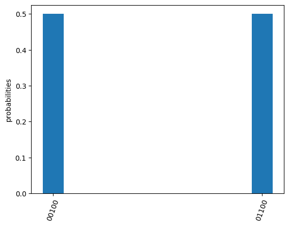
If you don’t want to plot the results for basis with zero probabilities,
set the parameter full in method
plot_probabilities to False. Note that this parameter is only valid for results returned by
the simulator.
A Subtle detail
There are two different conventions when writing a computational basis
as a bit-string. That is, for example, to denote the state where only
the first qubit is excited, some may write 10…000 while others use
000…01. This subtle detail sometimes causes confusion and even serious
error in computation. The following experiment demonstrates conventions
used in pyquafu.
from quafu import QuantumCircuit, simulate

n = 3
qc = QuantumCircuit(n)  # |000>
qc.h(0)  # |100> + |000>
qc.measure()

res = simulate(qc)
res.plot_probabilities()
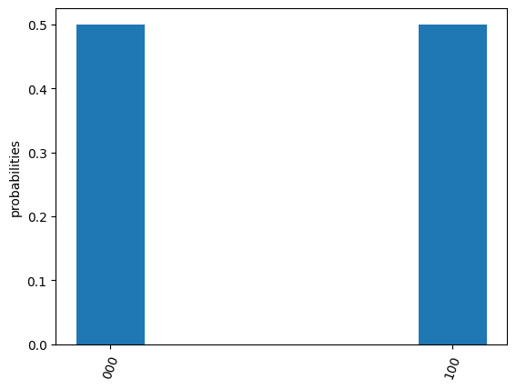
Here you see that in pyquafu, counts obeys so-called
‘big-endian’. However, for some historical reasons, the state-vector use
small-endian instead.
res = simulate(qc)
print(res.get_statevector()[:2])
state_tensor = res.get_statevector().reshape(tuple(n*[2])).transpose([-3, -2, -1])
print(state_tensor[0, 0, 0])
print(state_tensor[0, 0, 1])
print(state_tensor[1, 0, 0])
[0.70710678+0.j 0.70710678+0.j]
(0.7071067811865475+0j)
(0.7071067811865475+0j)
0j
If this is not the convention you are used to, ndarray.transpose may
help
state_tensor = state_tensor.transpose(tuple(range(n-1, -1, -1)))
Measure observables
Quafu provides measuring observables with an executed quantum circuit.
You can input Pauli operators that need to measure expectation values to
the submit <apiref/#quafu.tasks.tasks.Task.submit>`__ method. For
example, you can input [[“XYX”, [0, 1, 2]], [“Z”, [1]]] to calculate the
expectation of operators \(\sigma^x_0\sigma^y_1\sigma^x_2\) and
\(\sigma^z_1\). The
submit <apiref/#quafu.tasks.tasks.Task.submit>`__ method will
minimize the executing times of the circuit with different measurement
basis that can calculate all expectations of input operators.
Here we show how to measure the energy expectation of the Ising chain
First, we initialize a circuit with three Hadamard gate
q = QuantumCircuit(5)

for i in range(5):
    if i % 2 == 0:
        q.h(i)

measures = list(range(5))
q.measure(measures)
q.draw_circuit()
q[0]  --H-- M->c[0]

q[1]  ----- M->c[1]

q[2]  --H-- M->c[2]

q[3]  ----- M->c[3]

q[4]  --H-- M->c[4]
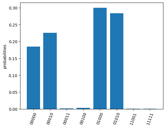
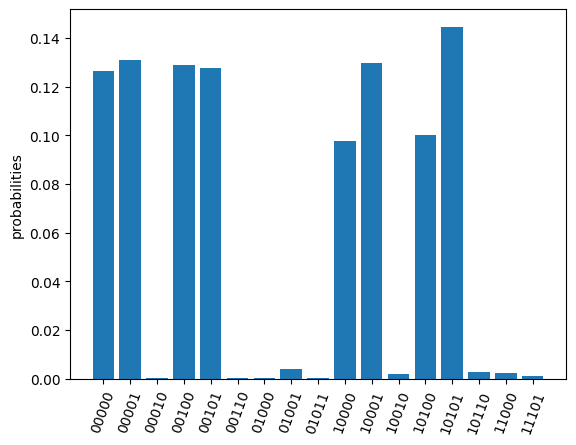
Next, we set operators that need to be measured to calculate the energy
expectation, and submit the circuit using
submit method
test_Ising = [["X", [i]] for i in range(5)]
test_Ising.extend([["ZZ", [i, i+1]] for i in range(4)])
res, obsexp = task.submit(q, test_Ising)
Job start, need measured in [['XXXXX', [0, 1, 2, 3, 4]], ['ZZZZZ', [0, 1, 2, 3, 4]]]
The function return measurement results and operator expectations. The measurement results only contain two ExecResult objects since the circuit is only executed twice, with measurement basis [[‘XXXXX’, [0, 1, 2, 3, 4]] and [‘ZZZZZ’, [0, 1, 2, 3, 4]]] respectively.
res[0].plot_probabilities()
res[1].plot_probabilities()
png
The return operator expectations (obsexp) is a list with a length
equal to the input operator number. We can use it to calculate the
energy expectation
print(obsexp)
g = 0.5
E = g*sum(obsexp[:5])+sum(obsexp[5:])
print(E)
[1.0, 0.046999999999999986, 1.0, 0.03699999999999998, 0.998, 0.00899999999999995, 0.08499999999999996, 0.08299999999999996, 0.008999999999999952]
1.7269999999999999
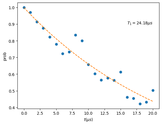
Submit task asynchronously
In the above examples, we chose opening python kernal and waiting for the result. You may also submit the task asynchronously. Here we use another example that measures the qubit decoherence time \(T_1\) to demonstrate the usage.
task = Task()
task.config(backend="ScQ-P10", shots=2000, compile=False, priority=2)
Prepare parameters of a group of tasks and send the task asynchronously.
ts = range(0, 21, 1)
names = ["%dus" %t for t in ts]
for name, t in zip(names, ts):
    q = QuantumCircuit(3)
    q.x(2)
    q.delay(2, t, unit="us")
    q.measure([2])
    res = task.send(q, name=name, group="Q3_T1")
Here the delay options will idle the target qubit 2 for a
duration t in the time unit us (microsecond) and do nothing. In
the send function, we set wait to false to execute the task
asynchronously, give each task a name by duration time and set all tasks
to a group named “Q3_T1”.
Now we can try to retrieve the group of tasks using the
retrieve_group
method.
group_res = task.retrieve_group("Q3_T1")
probs = [res.probabilities["1"] for res in group_res]
Group:  Q3_T1
task_id              task_name      status
326564501AF5CF47     0us            Completed
32656450226701BD     1us            Completed
326564502A80CC5D     2us            Completed
3265645032D98C32     3us            Completed
326564503AEFE7EA     4us            Completed
326564600CFE2817     5us            Completed
3265646014FFEA5F     6us            Completed
326564601C2E9597     7us            Completed
32656460240A93E6     8us            Completed
326564602C15CFFB     9us            Completed
3265646033EEBD20     10us           Running
326564603B1A478D     11us           In Queue
3265647006C96D3D     12us           In Queue
326564700F71B85A     13us           In Queue
32656470204A3472     14us           In Queue
32656470384DCD98     15us           In Queue
3265648004FB6BCF     16us           In Queue
326564800DA63F54     17us           In Queue
3265648022DAC675     18us           In Queue
3265648036F7EA24     19us           In Queue
326564901AB566FF     20us           In Queue
Once all the tasks are completed, we can do the next step to get \(T_1\).
group_res = task.retrieve_group("Q3_T1")
probs = [res.probabilities["1"] for res in group_res]
Group:  Q3_T1
task_id              task_name      status
326564501AF5CF47     0us            Completed
32656450226701BD     1us            Completed
326564502A80CC5D     2us            Completed
3265645032D98C32     3us            Completed
326564503AEFE7EA     4us            Completed
326564600CFE2817     5us            Completed
3265646014FFEA5F     6us            Completed
326564601C2E9597     7us            Completed
32656460240A93E6     8us            Completed
326564602C15CFFB     9us            Completed
3265646033EEBD20     10us           Completed
326564603B1A478D     11us           Completed
3265647006C96D3D     12us           Completed
326564700F71B85A     13us           Completed
32656470204A3472     14us           Completed
32656470384DCD98     15us           Completed
3265648004FB6BCF     16us           Completed
326564800DA63F54     17us           Completed
3265648022DAC675     18us           Completed
3265648036F7EA24     19us           Completed
326564901AB566FF     20us           Completed
import matplotlib.pyplot as plt
from scipy.optimize import curve_fit
def func(x, a, b):
    return a*np.exp(-b*x)

paras, pconv = curve_fit(func, ts, probs)
plt.plot(ts, probs, "o")
plt.plot(ts, func(ts, *paras), "--")
plt.xlabel("$t (\mu s)$")
plt.ylabel("prob")
plt.text(16, 0.9, r"$T_1=%.2f \mu s$" %(1/paras[1]))
Text(16, 0.9, '$T_1=24.18 \\mu s$')
Note that group_name and submite history are kept in the task
object only when python kernal is running. For data persistence, we
provide TaskDatabase which use qslite3 as the backend. It may
help you to save task information to your local computer.
We would not devote too much into developing TaskDatabase since the
web-backends will prodive more powerful and convenient usages in the
future. However, if you are interested in manipulating database freely
by qslite3, we do provide
tutorial
for a quick start.
from quafu.tasks.task_database import QuafuTaskDatabase, print_task_info

with QuafuTaskDatabase() as db:
    for res in group_res:
        db.insert_task(res.taskid, res.task_status, group_name="Q3_T1", task_name=res.taskname, priority=2)
    print('Tasks info stored')
    print("Task list:")
    for task_info in db.find_all_tasks():
        print_task_info(task_info)
        break  # this is to avoid demo too long, you may cancel this line to view the whole info
Tasks info stored
Task list:
Task ID: 326564501AF5CF47
Group Name: Q3_T1
Task Name: 0us
Status: Completed
Priority: 2
Send Time: None
Finish Time: None
------------------------
Finally, you can also retrieve a single task using its unique
task_id, and download all the historical tasks in
Quafu webpage.
res_20us = task.retrieve("1663B8403AE76050")
print(res_20us.probabilities)
{'0': 0.662, '1': 0.338}
Advanced usage
We offer some methods to build a quantum circuit more efficiently.
Apply the same gate repeatedly
Could use the power() method to apply the same gate consecutively.
import numpy as np
import math
from quafu import QuantumCircuit, simulate
from quafu.elements.element_gates import *

q = QuantumCircuit(2)
q << HGate(0)
q << HGate(1)
q << U3Gate(1, 0.2, 0.1, 0.3)
q << U3Gate(1, 0.2, 0.1, 0.3)
q << RYYGate(0, 1, 0.4)
q << RYYGate(0, 1, 0.4)
q << RXGate(0, 0.2)
q << RXGate(0, 0.2)
q << CRYGate(0, 1, 0.23)
q << CRYGate(0, 1, 0.23)

# Create another circuit using `power` method
q1 = QuantumCircuit(2)
q1 << HGate(0)
q1 << HGate(1)
q1 << U3Gate(1, 0.2, 0.1, 0.3).power(2)
q1 << RYYGate(0, 1, 0.4).power(2)
q1 << RXGate(0, 0.2).power(2)
q1 << CRYGate(0, 1, 0.23).power(2)

sv1 = simulate(q).get_statevector()
sv2 = simulate(q1).get_statevector()

# Check equivalence of two circuits
assert math.isclose(np.abs(np.dot(sv1, sv2.conj())), 1.0)
Join two quantum circuits
Use the join() method to merge two different quantum circuit.
from quafu import QuantumCircuit, simulate
from quafu.elements.element_gates import *

q = QuantumCircuit(3)
q << (XGate(1))
q << (CXGate(0, 2))
q1 =  QuantumCircuit(2)
q1 << HGate(1) << CXGate(1, 0)

# This extends the circuit `q` to 4 qubits,
# and apply `q1` to the 3rd and 4th qubit of `q`
q.join(q1, [2, 3])
q.draw_circuit()
q[0]  -------*-------
             |
q[1]  --X----|-------
             |
q[2]  -------+----+--
                  |
q[3]  --H---------*--
Reverse a quantum circuit
Use the dagger() method to reverse a quantum circuit.
import numpy as np
import math
from quafu import QuantumCircuit, simulate
from quafu.elements.element_gates import *

q = QuantumCircuit(3)
q << HGate(0)
q << HGate(1)
q << HGate(2)
q << RXGate(2, 0.3)
q << RYGate(2, 0.1)
q << CXGate(0, 1)
q << CRZGate(2, 1, 0.2)
q << RXXGate(0, 2, 1.2)

# Now create a reversed circuit of q
q1 = QuantumCircuit(3)
q1 << RXXGate(0, 2, -1.2)
q1 << CRZGate(2, 1, -0.2)
q1 << CXGate(0, 1)
q1 << RYGate(2, -0.1)
q1 << RXGate(2, -0.3)
q1 << HGate(0)
q1 << HGate(1)
q1 << HGate(2)

# Check equivalence
sv0 = simulate(q.dagger()).get_statevector()
sv1 = simulate(q1).get_statevector()
assert math.isclose(np.abs(np.dot(sv0, sv1.conj())), 1.0)